Data mining and analyzing the information found in a CMMS can lead to the ability to predict machinery failures
The idea of using reliability data to plan maintenance and future investments is quite appealing to many maintenance managers, but the topic seems to polarize opinions. Some people feel that with the help of software tools, historical maintenance data can lead to a good prediction mechanism for future failure behavior. Others dismiss the idea, feeling that the data available is too poor for serious prognoses.
The reliability engineering literature and many scientific papers don’t address this issue nor do they provide concrete examples of what levels of data are acceptable and how wide the margin of error will be. For these reasons, ABB Full Service and the ABB Corporate Research Life Cycle Science group decided to conduct a case study. The goal was to see whether a statistical analysis of CMMS data could be used as decision support for maintenance and investments. This article summarizes our findings and conclusions.
Overview
We tested several commercial reliability engineering tools. The case study site was a paper mill with a full service contract - all service activity was outsourced. The data used for the reliability calculations were taken from the site’s CMMS.
[pullquote]The specific equipment used in the study had a well-documented history in the CMMS with a number of entries in the single digits for each failure mode during the past three years. The data quality was generally good with only a few minor uncertainties. The equipment was considered troublesome in that it was clearly not “as good as new” after repairs. Instead, the intervals between failures seemed to be decreasing. The question arose whether it was possible to predict the approximate time of future failures and to make a cost/benefit analysis to determine whether a replacement was cheaper than future repairs.
Objective
Given the relatively thin database, it was clear that there would be inaccuracies. The goal of the study was to find evidence for answers to the important questions.
Can trends in equipment failures attributable to repairs be identified and are these trends pronounced enough to justify investments? In other words, is there a way to estimate the effect of multiple repairs on future times to failure?
Regardless of the existence of trends, can reliability analyses based on the data found in a CMMS system provide a good estimate of failure behavior? A particular focus lies on the amount of data - is there enough information to attempt such estimation or will the error margin be too high? Can the failure behavior estimation be used to schedule preventive maintenance activity and inspections? Can simulations provide a good prediction of future cost to use as a basis for maintenance budget planning?
Case study approach
To find answers to these questions, we chose the following approach. As a first step, we retrieved data from the CMMS and complemented it with other information. The main result was a list of times between failure (TBF) and times to repair (TTR). The TBFs and TTRs were used to determine the proper failure and repair time distribution functions. We relied on a commercial software tool to suggest a distribution function and to calculate its variables.
For the imperfect repair model, we calculated an age reduction factor using the so-called “Kijima II” method. Instead of a perfect repair that resets the age to zero, the imperfect repair model applies a factor to the age at the time of failure and continues the aging process with this “virtual age.”
We used a commercial simulation tool to build a simulation model of the critical system components based on the reliability curves and age reduction factors. We used the model to compare different scenarios:
- Investment: We compared the cost of an investment and the resulting effect on maintenance using a scenario that assumed nothing was changed. We tested both perfect and imperfect repairs.
- Maintenance planning: We compared maintenance strategies, which consisted of different combinations of inspections and preventive measures. The simulation tool provided some suggestion on what intervals and measures to use.
Determining the distribution functions
The commercial tool provided a suggestion for both the type of the distribution function and its variables based on the data taken from the CMMS. The failure distributions the software calculated had an acceptable value for the correlation coefficient and goodness-to-fit test (Chi-square or modified Kolmogorov-Smirnoff), which seemed to suggest a low margin of error for the final calculation. We also used the Kijima II method to determine the age reduction factors to represent the deterioration that multiple repairs cause.
From a theoretical standpoint, some of the suggested distributions were surprising as they indicated decreasing failure rates for mechanical components that typically are at least constant if not increasing because of wear-out.
For example, our model suggested that a transmission chain would get more reliable over time, the rate of breakage decreasing with age. For this reason, we also used the distribution functions recommended by theory with the same field data. The rationale was to test how great the effect of a “wrong” distribution function was.
Indeed, the choice of distribution had great effect on the simulation results. For example, the same data could lead to increasing and decreasing failure rates based on whether we used a Weibull 2 or Weibull 3 distribution. This difference has a great effect on preventive maintenance measures, especially preventive replacement of equipment.
Besides analyzing existing data, we also tried to determine the possible effect of errors in the CMMS using two pragmatic tests. First, we modified the CMMS data to simulate mistakes and gaps in the database. Second, we used “reverse-engineered” distribution functions as described below. The new functions were tested in the simulation to see their effect on the final result.
Simulation of systems under observation
Using the distribution functions and age reduction factors determined in the first step, we performed several simulations. We analyzed the behavior for all three subsystems both with and without age reduction to answer the questions formulated for the case study.
The simulations that answered the investment questions provided a clear answer for all three cases. However, it was surprising to see that the age reduction factors didn’t really cause a major increase in the number of failures. This was unexpected, as the local team had experienced a steady decline and expected far longer repair intervals after an “age reset” based on the behavior of similar equipment.
The simulation tool also gave some advice on the inspection intervals and preventive measures. For example, the simulation suggested we shorten the inspection interval for a chain that wasn’t very expensive to check as opposed to the downtime cost caused by its failure. On the other hand, a rather expensive preventive measure on a motor was identified as cost-ineffective as opposed to the repair and downtime cost.
To test the effect of wrong CMMS data, we performed one calculation with a modified data set for a motor in which we omitted one work order entry. The effect of this change was quite high. In fact, the difference it made to the total cost of ownership was as high as the effect of a replacement with a new machine. This means that the “noise” a single missing entry introduces has the potential to mask the effect of a decision under analysis. In the opposite case — the addition of a wrong dataset — the effect was less strong, but still not negligible.
Also, the results of using the “reverse-engineered” curves in the simulation were quite remarkable. Ideally, using a sample of random numbers based on a known distribution to re-calculate its variables should lead back to the original function, or at least a similar one. That means that different samples of the same function should result in approximately the same number of failures and, therefore, cost in the simulation.
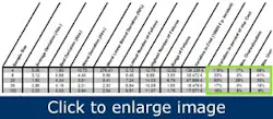
As a test, we selected five groups of samples of the same size from the same distribution function. The rows in Table 1 show the same test performed for different sample sizes ranging from 4 to 100 elements. We found that the resulting distributions differed widely. As a result, the number of expected failures ranged widely (6.45 to 9.99 in the case of eight CMMS entries). It’s interesting to note that the variation from random error is a lot higher than the effect calculated for a new investment. The results only stabilize when the sample size goes to 100 or more.
Table 1. Variations in Samples.
While these results seem quite disheartening, one must be careful not to jump to any conclusions, as this is only one case and not a comprehensive study. However, we feel confident to make several statements regarding our initial questions.
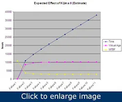
It’s our impression that the age reduction factors, no matter how they are determined, don’t help to identify required investments. In hindsight, this is not so surprising when one looks at Figure 1. After the first application of the age reduction factor, the age more or less stays constant. As a result, the MTBF is also quite constant.
Figure 1: Expected effect of Kijima II for the drive chain.
The data requirements for a good failure-probability prediction are far too high for any site with a scope that’s similar to our pilot study. The available failure data for a particular item must have at least 100 entries to be meaningful. The “quality indicators” such as the Chi-square test give false security. However, they can only show us how well the proposed curve fits our sample points and not how representative these points are for the actual distribution function.
While the suggested changes to the maintenance schedule all seemed plausible, we found that they’re too plausible. In other words, we don’t need a complex simulation and could have used a simple spreadsheet to come to the same conclusions. An explanation is that inspection suggestions are more influenced by ratio of downtime cost to inspection cost and time between first symptoms and actual failure than by the exact MTBF value.
Overall, while we feel that reliability tools have their uses, we think a careless application will do more harm than good, especially if your case is similar to ours. Even with poor data, one can construct seemingly perfect distribution curves and reach results that are heavily influenced by random factors as opposed to empirical facts.
Ralf Gitzel is scientist in the Life Cycle Science Group at ABB in Ladenburg, Germany. Contact him at [email protected].


